Mapping in D3

To make a map in D3, we must first start with a file that has cartographic information. We can then convert this for use in D3 or other software tools. Some of the most common formats of cartographic data files:

• ESRI Shapefile — This comes as a .zip file. When you extract it, it will contains multiple files required for calculating the cartographic coordinates, projection, and other metadata. These files are mostly used with a GIS software program, like ArcGIS or it’s free open source alternative, QGIS. This is the most common data format of maps in the GIS world, and generally you will start with this type of file. We will need to covert it to a format more friendly to JavaScript and web software.
• KML/KMZ or XML — These are formats that use XML (a generic HTML) to store the data. The KML format (and its identical, but compressed version KMZ) is mostly used by Google Earth and Google Maps for storing cartographic data.
• GeoJSON — This is a JSON format that is a specific standard for storing cartographic features. The GeoJSON website outlines the specification requirements for displaying shapes, lines, and other features.
• TopoJSON — Similar to the above GeoJSON, but it’s much more compact and efficient. GeoJSON files can often become very large and very process intensive. Designed by Mike Bostock, TopoJSON was aimed for efficiency without losing much quality. It’s designed to be used for any type of shape topology, not just cartographic purposes.

Projections

Before we begin, it’s also important to understand how map projections work. Projections is the cartographic science of taking a 3D shape, like a sphere, and representing it as a 2D plane surface.

D3 offers several choices for how to display map projections.

Process Overview

The first steps in the process is to convert our cartographic data as a topojson. This is the format most ideal with D3 and will give us the best results. The process will vary depending on what you start with. In most cases, using the tools shown in this page will work with different starting files.

The goal is to convert the file to an EPSG:4326 coordinate system, or verify that it is already set to this. This will use standard latitude and longitude coordinates for all the points in your shape.

Step 1: Starting with a Shapefile

In this example, we will start with a shapefile of election precincts in Contra Costa County, California. Most shapefiles are available for download on the websites of local government agencies. This one was provided by the elections office of Contra Costa County.

Download Election Precincts for Contra Costa County (.zip)

Optional: Viewing the file in Mapshaper.org

We can view the file in MapShaper. This process is just informational, so we can see what it looks like. Clicking the “i” icon and hovering over the various features of the map helps us understand the type of data associated with each feature.

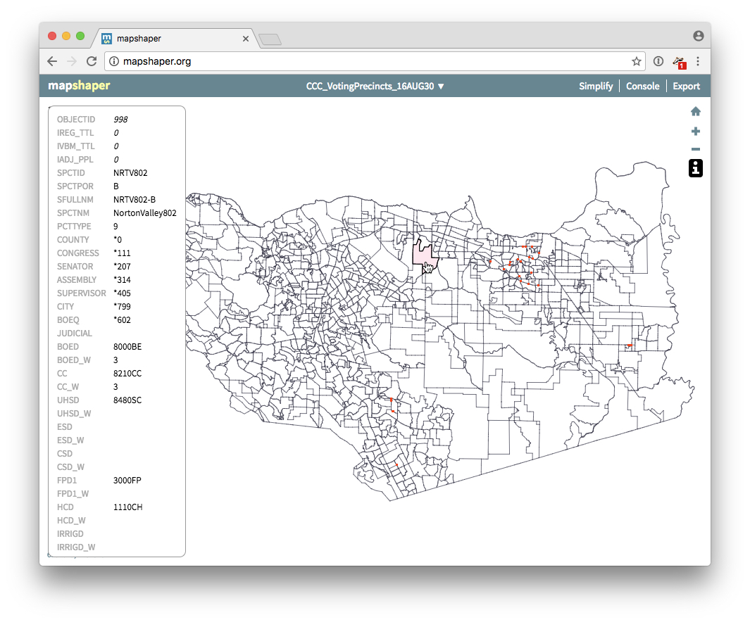
Note: Mapshaper has the ability to export files as GeoJSON and TopoJSON. Sometimes this would be OK to perform at this time. But in our example, we won’t use MapShaper to do this right now, because our shapefile is in a different coordinate system other than EPSG:4326. We need to first convert it before exporting as TopoJSON!

Step 2: Checking the Embedded Coordinate System

Shapefiles have a coordinate system embedded in them. You can think of this like an Cartesian X and Y grid, but where the values have different meaning depending on the type of map and where you got your shapefile.

D3 likes EPSG:4326, because it uses a common latitude/longitude coordinate system. Some shapefiles might already be setup with EPSG:4326, so this step can be optional.

To verify the coordinate system of your shape file, upload the .prj file to Prj2epsg.org. The .prj file is inside your shapefile .zip. You’ll need to unzip the shapefile temporarily so we can document which coordinate system it’s using. Make sure you keep the files intact and don’t throw away your .zip file just yet, we’ll still need it!

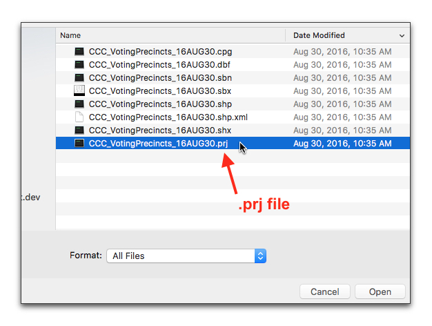
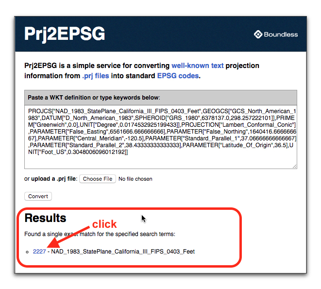
We can see from the results, our shape file is embedded with EPSG:2227 coordinates. We need to convert it from EPSG:2227 to EPSG:4326!

Step 3: Converting to EPSG:4326

Next, we’ll visit the Ogre to Ogre (ogr2ogr) web client to convert our file to the correct EPSG:4326 coordinate system.

Ogr2ogr is a free command line program that can be installed though a package called GDAL, or through Homebrew.

However, there is an easier way using a free online web client and it doesn’t require installing anything. The web client should work for most applications. The drawback is that there are limited options for conversion, and there is a file size limit. Should either of these be an issue, then you’ll need to install ogr2ogr manually and run the following command from the Terminal program (You’ll need to do this from the folder where your shapefile is located.):

ogr2ogr -f GeoJSON output_file.geojson -t_srs EPSG:4326 your_shapefile.shp

For everyone else using the web client version, just visit: ogre.adc4gis.com. You’ll need to upload the entire shapefile .zip file.

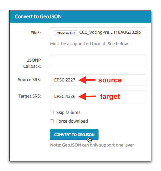
With some browsers like Chrome, it may output the GeoJSON file as text in your window. Simply press Command (Ctrl on PC) + S to save the file with a .json file extension. The name of the file will be used later, so make sure the file name has no spaces and is well understood.

Step 4: Converting to TopoJSON

Next, we’ll upload our GeoJSON file to Mapshaper, and convert it to TopoJSON. Visit the Mapshaper website, and upload your GeoJSON file that you saved from ogr2ogr (not the original .zip shapefile!).

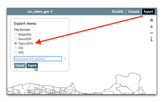
Advanced Users Note: If you already know the metadata you want to associate with each feature, you can add id-field= to the command line options during export and it will become the “id” property of each feature. In this current Contra Costa County Precinct, for example, we can put id-field=SPCTNM so that the SPCTNM field, which is the precinct name, will be associated with each feature’s id. Without doing this, all metadata will still be preserved.

Optional: If you wanted to use the command line to cover to topojson, you’d need to install it first through NPM, a package manager for installing Node.js applications.

To install topojson, type the following command in teriminal (after installing npm). It will require administrative password.

sudo npm install -g topojson

After installing, you’ll have the geo2topo command available to you. This allows you to convert from TopoJSON to GeoJSON and vice versa.

The command syntax format is geo2topo featureName=[inpput file name] > [output file name].

geo2topo objects=input.json  > output.json

Simplifying the topojson file

In some cases, you may end up with a very large file still, especially if there are lots of features in your file. The topojson program comes with a utility to reduce the size of the file, but simplifying some of the lines and arcs.

toposimplify -p 1 -f -o output.topojson input.topojson  

There is also a utility called topoquantize, which will round the numbers in the file to better optimize loading. The first argument is a power of to quantize. Typically 1e4, 1e5 or 1e6 is chosen. Over quuantizing your json file will result in very odd looking map.

topoquantize 1e5 -o ouput.topojson input.topojson

Step 5: Building a D3 Map

Let’s start with a very basic starter template:

<!DOCTYPE html>
<html>
<head>
    <meta charset="utf-8">
    <title>D3 Map Example</title>
</head>
<body>


<script src="https://d3js.org/d3.v5.min.js"></script>
<script src="https://unpkg.com/topojson@3"></script>
<script>


</script>
</body>
</html>

Notice we’re loading in two D3 libraries; the main library, and one topojson sub-library. In the <script> tag, we’ll setup our basic SVG, and setup a path function which will draw our map.

Note: The .parallels([34,40.5]) and .rotate([120,0]) functions are using the Albers EPSG:3310 projection for California. Looking at the “Well Known Text or WKT” on the linked website will tell you these values for your own state or region.

var svg = d3.select("body")
    .append("svg")
    .attr("width", 960)
    .attr("height", 600);


d3.json("ccc_precinct_topo.json").then(function(mapData){

    console.log(mapData);

    var contraCosta = topojson.feature(mapData, {
        type:"GeometryCollection",
        geometries: mapData.objects.output_file.geometries
    });

    //fitExtent has the padding (20,20) and box size (960,600)
    var projection = d3.geoAlbers()
      .parallels([34, 40.5])
      .rotate([120, 0])
      .fitExtent([[20,20],[960,600]], contraCosta);

    var path = d3.geoPath()
        .projection(projection);

    svg.selectAll("path")
        .data(topojson.feature(mapData, mapData.objects.ccc_voters_geo).features)
        .enter()
        .append("path")
        .attr("d", path)
        .attr("stroke", "#000000")
        .attr("fill", "#ffffff");

});

The above code assumes that you named your TopoJSON file ccc_precinct_topo.json. Also, we need to figure out what the features object is in your data. If you followed this tutorial, Mapshaper would have made the object property name the same as the file name of your GeoJSON file (the one you exported from ogr2ogr). You can also find this out by looking at your console data, which we exported using console.log(mapData).

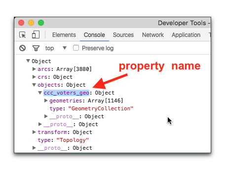
Note that in this example our property name is ccc_voters_geo (as seen in the above image. Yours may be different!). We need to use this in our data() function:

.data(topojson.feature(mapData, mapData.objects.ccc_voters_geo).features);

Change your mapData.object.[name of property] to match your console.

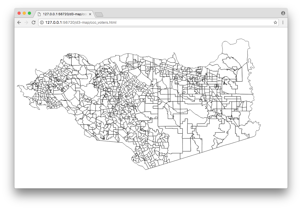
You should see a map appear:

Step 6: Loading Other Data to Color the Map Features

Next, let’s load a .csv (spreadsheet data) so that we can color-code these precincts. We’ll use the latest election results from the 2016 primary elections:

2016 Primary Election Results (Excel)
2016 Primary Election Results (CSV)

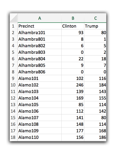
Let’s make a map to find out who voted for Hillary Clinton vs Donald Trump. I’ve included both the Excel file and .csv file. We will use the .csv in this tutorial. The Excel file is included in case anyone wanted to experiment and try analyzing other candidates.

Step 7: Loading in multiple data files using Promise function

Sometimes we need to load in multiple data files simultaneously. JavaScript has a utility called Promise for doing just this.

Promise.all([
  d3.json("ccc_precinct_topo.json"), 
  d3.csv("CCC_Primary_results.csv") 
])
.then(function(data){

//data[0] will be our topo json
//data[1] will be our csv results, (because it was listed second)

});

We should relabel our data variables to reflect loading in two files. At this point, our JavaScript should look like this:

var svg = d3.select("body")
    .append("svg")
    .attr("width", 960)
    .attr("height", 600);

var projection = d3.geoMercator()
    //center of your map
    .center([-121.979141, 37.940119])
    .scale(60000);//zoom factor

var path = d3.geoPath()
    .projection(projection);

  
Promise.all([
  d3.json("ccc_precinct_topo.json"), 
  d3.csv("CCC_Primary_results.csv") 
])
.then(function(data){

    svg.selectAll("path")
        .data(topojson.feature(data[0], data[0].objects.ccc_voters_geo).features)
        .enter()
        .append("path")
        .attr("d", path)
        .attr("stroke", "#000000")
        .attr("fill", "#ffffff");
});

Step 8: Understanding d3.map() collections

In order to pair the data from our spreadsheet to the shapefiles, we’ll need a special object variable. D3 has something called d3.map() built just for this purpose. It’s a really simple function that allows you to create an object, and set the keyword for this object. In addition, there are some functions for retrieving the data based on the keyword you set. Let’s look at an arbitrary example:

//just an example, don't use this in your map

var my_map = d3.map(); //we create a d3.map() collection object

//using the set function, we can associate data with keywords
my_map.set("dog", 32894);
my_map.set("cat", 54334);
my_map.set("mouse", 32452);

//later on, if we want to get the data, we can retrieve it by keyword
my_map.get("dog"); //returns 32894
my_map.get("cat"); //returns 54334
my_map.get("mouse"); //returns 32452

This gives us a general idea of how d3.map() works, but it’s not practical to create a map of every variable in our dataset.

In a real-world scenario, we would use map collections like this:

//load data from a csv
d3.json('animal_data.csv').then(function(data){


/* What our data variable would look like if we analyzed it
[
  {name: "dog", value: 32894},
  {name: "cat", value: 54334},
  {name: "mouse", value: 32452}
]
*/

//the d3.map allows us to pass in the "data" variable as first argument
//and the second argument is a function that returns each "key", or value
//that we specify to get back associated data.
var my_map = d3.map(data, function(d){ return d.name; });

//later on, if we want to get the data, we can retrieve it by keyword
my_map.get("dog"); //returns 32894
my_map.get("cat"); //returns 54334
my_map.get("mouse"); //returns 32452

});

So, now that we generally understand how maps work, let’s use it in our example.

  var election_map = d3.map(); //create the map object

  data[1].forEach(function(d){
    //use the .set() function to associate results with each precinct
    election_map.set(d["Precinct"], {"trump" : d["Trump"], "clinton": d["Clinton"]});
  });

What this does is allows us to recall either candidate’s results based on the precinct name.

election_map.get("Alhambra101"); // will return object {trump: 11, clinton: 18}

Since some the shapefile data has precinct names associated with each shape, when we make our D3 map, we can reference this election_map variable to extract the voter data.

Step 9: Integrating the d3.map() into our code

Because we are loading in the data through an AJAX method (meaning, we’re fetching the data from an external file), we need to convert all of the strings into numbers. This process is called coercion. We can coerce a string into a number by adding a plus symbol + before the variable. So, d["Trump"] = +d["Trump"] means it’s reassigning the variable to the number version of itself.

Promise.all([
  d3.json("ccc_precinct_topo.json"), 
  d3.csv("CCC_Primary_results.csv") 
])
.then(function(data){

    var election_map = d3.map(); //create the map object

    data[1].forEach(function(d){
      //use the .set() function to associate results with each precinct
      d["Trump"] = +d["Trump"];
      d["Clinton"] = +d["Clinton"];
      election_map.set(d["Precinct"], {"trump" : d["Trump"], "clinton": d["Clinton"]});
    });

// Note: rest of the code omitted here...
});

Step 10: Setting the Scales

We need a scale from red to blue. We are going to use one of d3’s Red-Blue chromatic scales, but we could have used our own.

In order to use the scale, we need to set an extent of our data… which value gives us the most red, and which value gives us the most blue. There are many ways to do this, and there are some ethical considerations. The degree of red or blue indicates data intensity, how many more votes in a particular district did one candidate get than another.

First, let’s calculate the extent by using d3.max() function. This function allows us to extract the maximum value in an array. It optionally takes a second argument, which is a function that can return a property from an object in the array.

For example, if I ran the following example:

d3.max([3, 5, 1, 4]);
//This would return 5, since 5 is the maximum value in the array.


d3.max(
  [
    {name:"Joe", age:32},
    {name:"Jill", age: 22},
    {name:"Jane", age:18}
  ],
    function(d){ return d.age;}
  );
//This would return 32, since it's the maximum value. 
//Notice the second argument allows us to return just the ages,
//and ignore the name property.

In our example, let’s extra the maximum values of votes for Clinton and Trump, but only when we subtract them from each other, so we can see the maximum value of votes MORE than each candidate got from any particular district.

//returns maximum number of votes MORE trump got than clinton in any given precinct
var trumpMax   = d3.max(data[1], function(d){ return d["Trump"] - d["Clinton"]; });

//returns maximum number of votes MORE clinton got than trump in any given precinct
var clintonMax = d3.max(data[1], function(d){ return d["Clinton"] - d["Trump"]; });

The return values with our practice dataset are:

Trump: 180
Clinton:440

If you imagine the vote distribution along a number line, with the maximum number of votes for Trump toward red, and maximum for Clinton in blue. It wouldn’t be an even distribution (at least, not in the San Francisco Bay Area).

So, we shouldn’t set our scales in such a way that the maximum number of votes trump got equates to the darkest shade of red. Otherwise, it will distort most of the precincts, showing them as a light shade of red, even if Clinton got more votes in those.

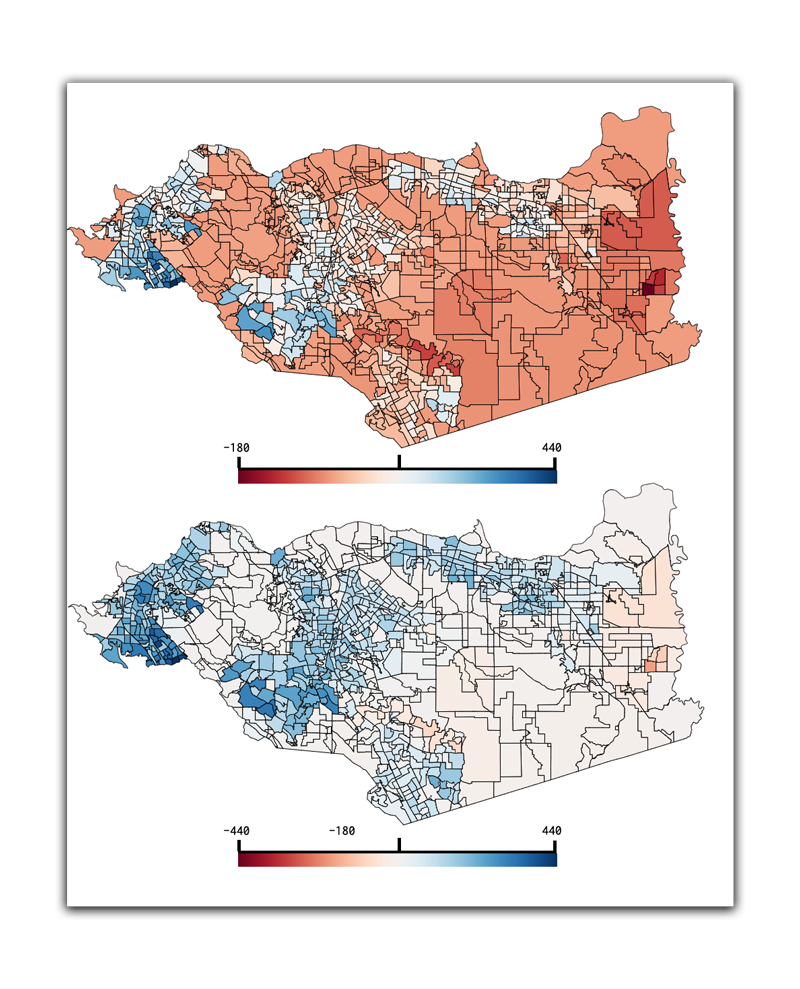
The bottom map is a more honest representation of the vote distribution. In Contra Costa County (a more liberal county in California), more voters voted for Clinton, which the exception of a few precincts colored in the a light shade of red. Those precincts only depict modest vote totals where Trump beat Clinton, so the intensity of the red doesn’t equate to the intensity of the blue shades where Clinton overwhelmed Trump in vote totals.

The final (proper) scales would now read:

var trumpMax   = d3.max(data[1], function(d){ return d["Trump"] - d["Clinton"]; });
var clintonMax = d3.max(data[1], function(d){ return d["Clinton"] - d["Trump"]; });

var colorScale = d3.scaleSequential(d3.interpolateRdBu)
  .domain([-clintonMax, clintonMax]);

Step 11: Adjusting our map code to color each precinct

Our fill code is based on the precinct Shapefile, which only has the name of the precinct associated with it.

For example, if you performed a console.log() on your fill code:

.attr("fill", function(d){ 
    
    console.log(d);

    return "#ffffff"
});

You would see each piece of the Shapefile (called “feature”) and the data associated with it.

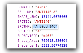
We can extract the name of the precinct using d.properties.SPCTNM. But how do we get the vote tallies? This is where we rely on our d3.map() function we setup earlier and saved into the variable election_map. We can use the election_map.get(d.properties.SPCTNM) function to retrieve the vote totals from each precinct.

.attr("fill", function(d){ 
    let precinct = election_map.get(d.properties.SPCTNM) || {trump:0, clinton:0};
    return colorScale(precinct["clinton"]-precinct["trump"]);
});

Our Shapefile contains a few precincts that aren’t in our data. So election_map.get(d.properties.SPCTNM) returns an “undefined” value. We can mitigate this by using a boolean OR operation trick, which means if it’s undefined, the alternative will be used.

//retrieve the vote counts OR if undefined, just return zero votes for each, 
//which will be in the middle of the color spectrum (gray)
election_map.get(d.properties.SPCTNM) || {trump:0, clinton:0};

Step 12: Final Code

The final code for the whole map is as follows:

<!DOCTYPE html>
<html>
<head>
    <meta charset="utf-8">
    <title>D3 Map Example</title>
</head>
<body>


<script src="https://d3js.org/d3.v5.min.js"></script>
<script src="https://unpkg.com/topojson@3"></script>
<script>

var svg = d3.select("body")
    .append("svg")
    .attr("width", 960)
    .attr("height", 600);

  
Promise.all([
  d3.json("ccc_precinct_topo.json"), 
  d3.csv("CCC_Primary_results.csv") 
])
.then(function(data){

    var contraCosta = topojson.feature(data[0], {
        type:"GeometryCollection",
        geometries: data[0].objects.output_file.geometries
    });


    var projection = d3.geoAlbers()
      .parallels([34, 40.5])
      .rotate([120, 0])
      .fitExtent([[20,20],[960,600]], contraCosta);


    var path = d3.geoPath()
        .projection(projection);

    var election_map = d3.map(); //create the map object

    data[1].forEach(function(d){
      //use the .set() function to associate results with each precinct
      d["Trump"] = +d["Trump"];
      d["Clinton"] = +d["Clinton"];
      election_map.set(d["Precinct"], {"trump" : d["Trump"], "clinton": d["Clinton"]});
    });
  
    var trumpMax   = d3.max(data[1], function(d){ return d["Trump"] - d["Clinton"]; });
    var clintonMax = d3.max(data[1], function(d){ return d["Clinton"] - d["Trump"]; });
  
    var colorScale = d3.scaleSequential(d3.interpolateRdBu)
      .domain([-clintonMax, clintonMax]);
  
    svg.selectAll("path")
        .data(topojson.feature(data[0], data[0].objects.ccc_voters_geo).features)
        .enter()
        .append("path")
        .attr("d", path)
        .attr("stroke", "#000000")
        .attr("fill", function(d){ 
            let precinct = election_map.get(d.properties.SPCTNM) || {trump:0, clinton:0};
            return colorScale(precinct["clinton"]-precinct["trump"]);
        });
});
  
</script>
</body>
</html>