Working with Data

Below is a tutorial on basic use of Google Sheets which we will do in class.

Written by Jeremy Rue

Introduction

A spreadsheet is a software program you use to easily perform mathematical calculations on statistical data and totaling long columns of numbers or determining percentages and averages.

And if any of the raw numbers you put into your spreadsheet should change – like if you obtain final figures to substitute for preliminary ones for example – the spreadsheet will update all the calculations you’ve performed based on the new numbers.

You also can use a spreadsheet to generate data visualizations like charts to display the statistical information you’ve compiled on a website.

This tutorial will focus on the use of the free application Google Spreadsheets. To use Google Spreadsheets, you will need to sign up for a free Google account. There are other spreadsheet software you can purchase, like Microsoft Excel. While this tutorial will focus primarily on Google Spreadsheet, most of its lessons will be applicable to any spreadsheet software, including Excel.

Spreadsheet Layout

To create a new spreadsheet in Google Spreadsheet, sign into your Google Drive account. Then click on the New button on the top left and select Google Sheets.

On your screen will appear a basic spreadsheet, divided into numbered rows and lettered columns.

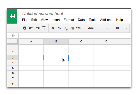
The rows and columns intersect to create small boxes, which are called cells.

Each cell is identified by its column letter and row number.

Thus the very first cell in the upper left-hand corner is called A1.

Just below A1 is A2. Just to the right of A1 is B1. Just below B1 is B2, and so on.

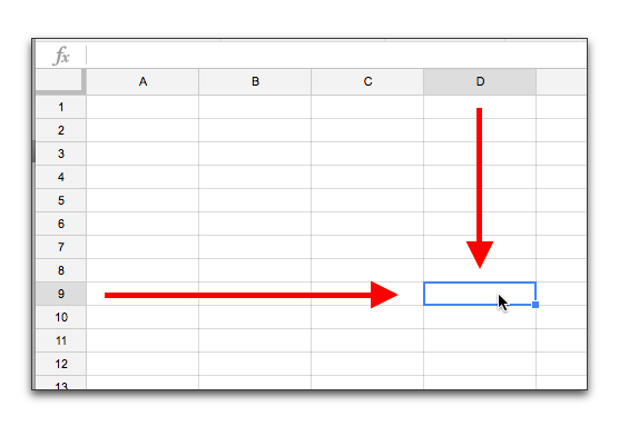
In the image below, for example, cell D9 is highlighted.

Setting the View Options

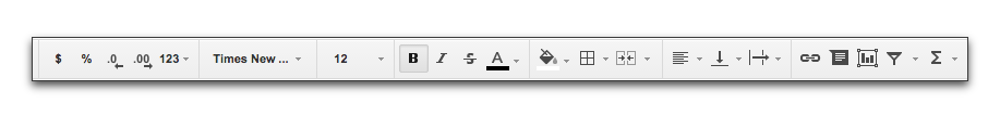
You can select some settings to change the view of the spreadsheet or display toolbars you frequently use, such as the one for entering formulas to make calculations.

To do this, in the menu at the top click on View and make sure there’s a check mark next to Formula Bar.

Entering Information in a Cell

You enter information into a spreadsheet program by typing it into each of the cells.

You can enter three different types of information into a cell:

• Numbers – so you then can perform mathematical calculations on them.
• Text – to identify what the numbers in the columns and rows represent, usually by typing headings across the top of the columns or on the left edge of the rows
• Formulas – to perform calculations on the numbers in a column or a row of cells.

To enter information into a cell, simply click on the cell and type in the information.

When you’re done, you can either press the enter/return key, which will take you down to the next cell, or the tab key, which will advanced to the cell to the right.

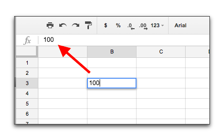
Each time you type information into a cell, you’ll notice the information also appears in the Formula bar, the box just above the columns and rows.

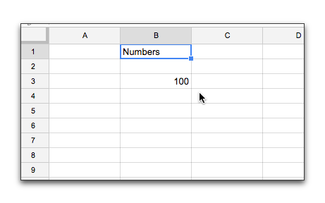
For example, if you click on cell:

B3

And type in the number:

100

You’ll see the number 100 displayed in the formula bar above.

Add Headings

To enter text headings for the various columns and rows to identify them, follow the same procedure as you would with entering numbers. Click on the cell, type in the name of a heading and press the enter/return key.

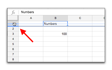
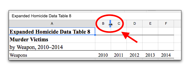
You can also “freeze” this header row, so it stays in the same place, even if you scroll down a long spreadsheet. To do this, grab the small bar in the corner of the spreadsheet area, and drag it down one row.

Importing Data Into a Spreadsheet

Many government agencies and private organizations provide data on their websites in a spreadsheet or other format that you can download onto your computer.

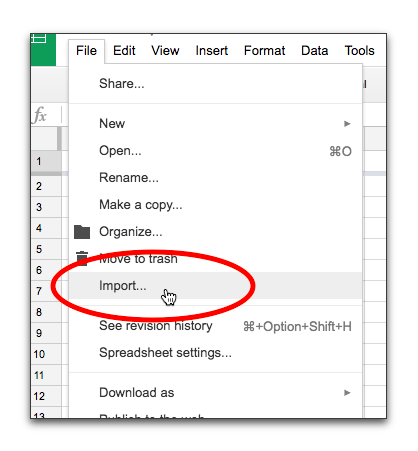
To import a spreadsheet, .csv or other file you’ve downloaded on your computer into a Google Spreadsheets, first create a new spreadsheet in Google Docs. Then in the menu at the top click on File … Import and then Browse and select the downloaded file.

Note: You also can import data on a website directly into a Google Docs spreadsheet. For instructions on doing that, see the section on Functions later in this tutorial.

Importing Sample Data

Let’s download some data to demonstrate how to import it into a Google Spreadsheets, and also to give us some sample data to use to show how to do calculations and use other features of a spreadsheet.

The FBI compiles national crime statistics, including data on the types of weapons used in homicides.

This data is in an Excel spreadsheet (.xls) file that can be downloaded from the FBI website and then imported into a Google Doc spreadsheet.

To download the file go to this FBI web page:

Expanded Homicide Data Table 8 (2010-2014)

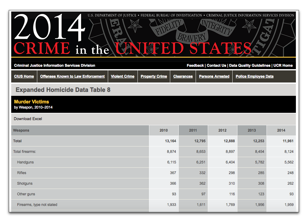
Click on the link at the top for:

Download Excel

The file will be downloaded onto your computer.

(if for some reason you have trouble downloading this file, you can click here to download the file from our website)

To import the file into a Google Docs spreadsheet, create a new spreadsheet and in the menu at the top click on:

File … Import

Click on the Browse button and navigate to the downloaded FBI file which is named expanded_homicide_data_table_8_murder_victims_by_weapon_2010-2014.xls. Google Spreadsheet also allows you to import data from your Google Drive. It may give you an option to replace existing data, or to create a new sheet. Choose the best option for your situation.

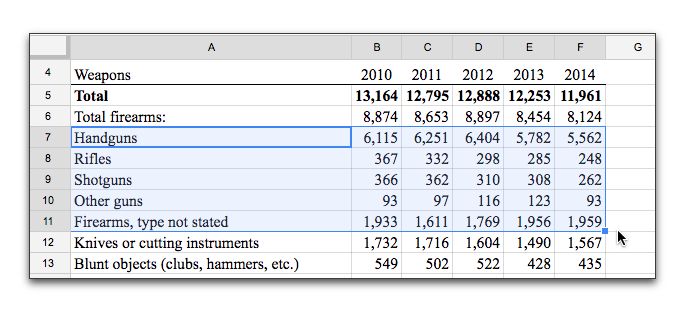
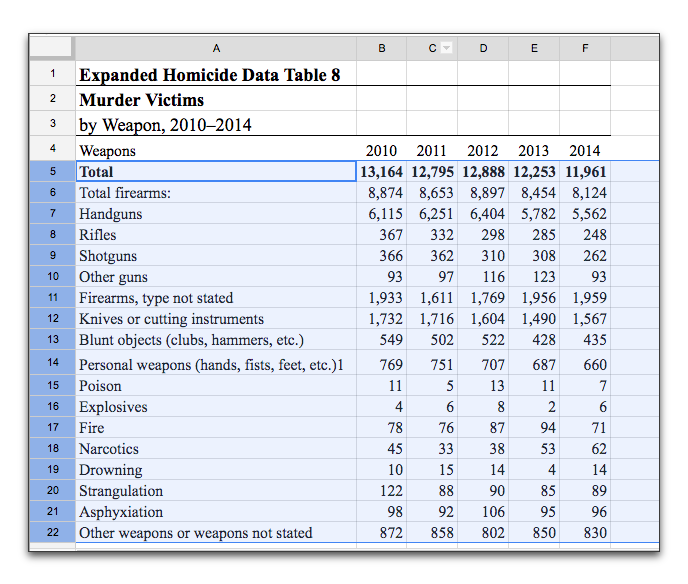
After a few seconds you should see a Google Docs spreadsheet that looks like this:

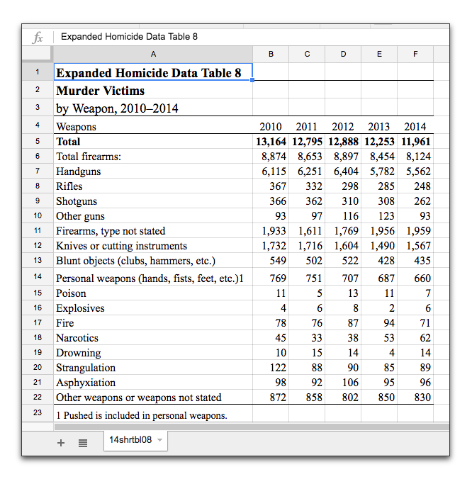
This spreadsheet shows the number of murder victims in each year from 2010 to 2014 in five columns, with the columns labeled by year in cells B4 to F4.

Below that the spreadsheet shows the weapon used in the murders in 17 rows of data, with the rows labeled by type of weapon in cells A5 (which is the overall total for all weapons) to A22.

Resizing Columns or Rows

You can improve the display of the data in a spreadsheet by increasing or decreasing the width of a column or the height of a row.

To change a column’s width, in the gray bar at the top of the spreadsheet where the letters of the columns are displayed, move your mouse cursor to the border between any two columns.

Note for Excel: if you narrow the width of a column displaying a number too much, you will see a series of pound signs displayed in the cell:

###

This doesn’t mean you’ve lost any data – you just made the column width too narrow to fit some of the numbers in the cells in that column.

You can also speed up the resizing of columns and avoid making them too narrow by moving your mouse cursor to the border separating two columns in the gray bar at the top and double-clicking on the border. This will automatically resize the column to the left, making it just wide enough to fit the longest entry on any row in that column.

Deleting or Adding Columns or Rows

You can get rid of unwanted data or other information by deleting rows or columns.

For example, in our sample spreadsheet of weapons used in homicides, we might want to get rid of row 23, which is just a footnote stating that one murder in which the victim was pushed to his/her death has been included in the “Personal weapons” listing in row 14.

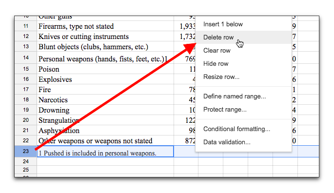
To delete a row, hover your mouse cursor over a row number in the gray area to the left, in this case row 23. Right click and in the pop-up menu select Delete row.

Use the same procedure for deleting a column.

If you want to add a column or row, again hover your mouse cursor over the appropriate column or row in the gray area above or to the left, right click and in the pop-up menu select one of the Insert options.

Formulas – Adding, Subtracting, Multiplying and Dividing

With a spreadsheet you can insert a formula that will instantly add, subtract, multiply or divide numbers in columns or rows. To do this you select a cell in a new column or row and then type in a formula.

A formula starts with an equals sign = that tells the spreadsheet you want to do a calculation.

A formula then has a symbol for what kind of calculation you want to perform (add, subtract, multiply, divide, etc.). The symbols a spreadsheet uses for calculations are:

• plus sign (+) for adding one number to another
• minus sign (-) for subtracting one number from another
• asterisk (*) for multiplying one number by another
• backslash (/) for dividing one number by another

Then you type in the letters/numbers for the cells (A1, A2, B1, B2, etc.) to which you want to apply the calculation, separated by the symbol for the type of calculation.

Adding Numbers in Columns

Let’s write a formula for adding together a series of numbers.

In the spreadsheet for types of weapons used in murders that we downloaded from the FBI website, the spreadsheet already included the total number of homicides in which any kind of firearm was used each year from 2010 to 2014. Those numbers are in row 6.

But what if these totals hadn’t been included in the original data and you needed to calculate them yourself using the spreadsheet (or if you wanted to use the spreadsheet to double-check the FBI’s calculations).

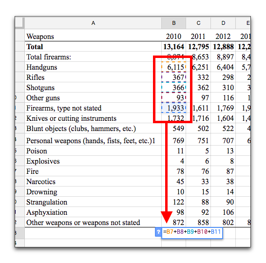
This would require totaling up for each year the column of numbers for the five weapon types in the spreadsheet:

• Handguns – row 7
• Rifles – row 8
• Shotguns – row 9
• Other guns – row 10
• Firearms, type not stated – row 11

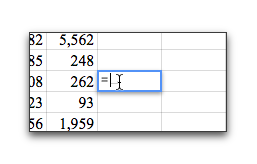
To do this we need to insert a formula for adding a series of numbers in a column. Let’s start by doing this for the year 2010. Click on cell:

B23

Which is in the column that shows the numbers for weapons used in 2010.

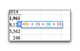
In that cell, type:

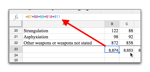
=B7+B8+B9+B10+B11

(note: the letters are not case sensitive. So for example so you could type in either B7 or b7)

You should type cell letters/numbers into a formula rather than the actual numbers.

That way if the numbers ever change (for example, if the FBI released updated murder weapon statistics for 2008), you won’t have to re-enter the new numbers in the formula. Instead you’d just type the updated numbers into the appropriate cells and the spreadsheet will apply the existing formula to the new numbers in those cells.

Applying a Formula to Multiple Cells

If we now wanted to calculate the total number of gun related homicides for the other four years, we could repeat the process of typing an addition formula into each cell in the rest of row 23. But a spreadsheet has a much faster way of accomplishing this – by letting you simply copy the formula to one or more of the other cells in the same row.

To do this, click on cell:

B23

Where we typed in our addition formula =B7+B8+B9+B10+B11.

Pass your mouse cursor over the bottom right corner of cell B23 and notice a small box where your cursor changes from an arrow pointer to a thin crosshairs.

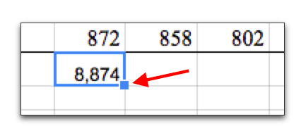
Click on that crosshairs, hold down your mouse button and drag your mouse to the right over the rest of the cells in row 23.

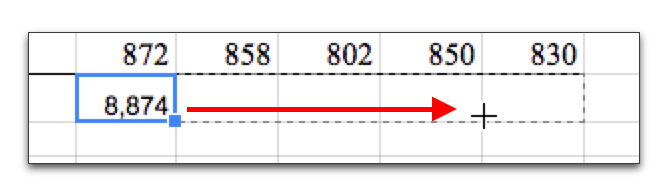
An outline will appear around the cells you’ve selected.

Continue dragging your mouse until you get to cell:

F23

Release your mouse button and the total number of homicides involving firearms for each year from 2010 to 2014 will appear in row 23.

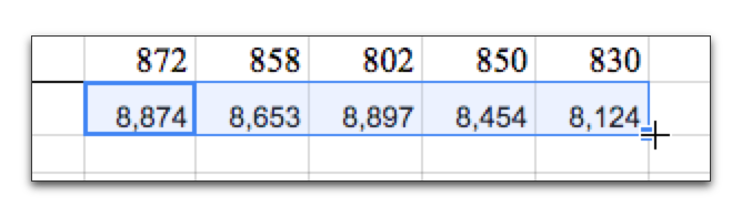
Which again confirms the totals in the original FBI spreadsheet in row 6.

The spreadsheet has calculated these totals for you by applying the formula you first typed in cell B23 to the rest of the cells in row 23.

The spreadsheet keeps the formula (addition) the same, but shifts the cell numbers as it applies the formula to the other cells to the right (so the formula in cell C23 is =C7+C8+C9+C10+C11, the formula in cell D23 is =D7+D8+D9+D10+D11, and so on).

Editing a Formula

When you type a formula into a cell and then hit the enter/return key, the formula will disappear, replaced by a number that’s the result of the calculation.

So how can you edit the formula?

There are two ways:

You can double click on the cell to display the formula in the cell and then edit or retype it there.

Or you can click once on a cell and use the Formula bar above to edit it.

If you click once on a cell that has a formula hidden in it (replaced by a number that’s the result of the calculation), the formula you originally typed will appear in the Formula bar above the columns and rows.

To edit the formula you can click in the formula bar where the formula for this cell is displayed. Then change the existing formula or type a new one into the Formula bar, press the enter/return key and the new formula will be applied and the numbers will be recalculated in the cell.

Understanding Cell Formats

Cells can display their data in many different ways. For example, you can format a cell to display data as currency, as a date, scientific notation, or several other formats. You can adjust this by highlighting a cell, and changing its format under the Format -> Number menu.

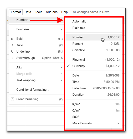
This can sometimes be counter-intuitive because the cell can appear differently than the data that’s actually in the cell. For example, in the case of currency format, the cell data could have several decimal places. But when formatting for currency, a dollar symbol will display and the cell will only show the hundredths place (2 decimal points), even if the actual data in the cell has is more exact and has more decimal points.

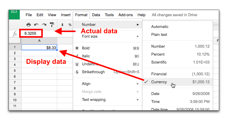
The way to understand what the actual data is in a cell is to look at the formula bar. This will sometimes show you the raw data. The cell format is generally used to make thing more human-readable. But sometimes this can be the cause of consternation, especially when using formulas. This could especially be tricky when using dates.

Percent Changes and Multiplying and Dividing

This next section will describe how to calculate a percent change between two numbers. A percent change is calculated by finding the difference between the two numbers, and comparing that difference by the first number.

In our spreadsheet on murder weapons, we can calculate how much each weapon increased or decreased between 2010 to 2014.

First click on cell G5 to the right of our existing data.

Type in the following formula:

=(F5-B5)/B5

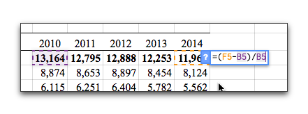
This is the formula for calculating the percent change between two numbers.

This formula tells the spreadsheet to find the difference of homicides by subtracting the total homicides in 2014 from 2010. After that, divides the results to the original value.

The backslash ( / ) is the symbol for dividing, while the asterisk ( * ) is the symbol for multiplying.

(Note: The parentheses in this formula are also important to define the correct order of operations.)

Now hit the enter/return key to see the final result of the percent formula in cell G5:

-0.09138559708

The total number of homicides by all types of weapons declined by 9.1 percent from 2010 to 2014. But to make it into a more human-readable format, we can change the data format of the cell to a percentage.

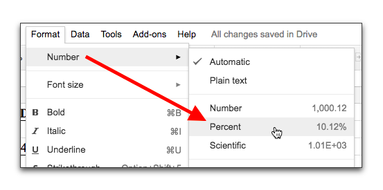
Now it will display as:

-9.14%

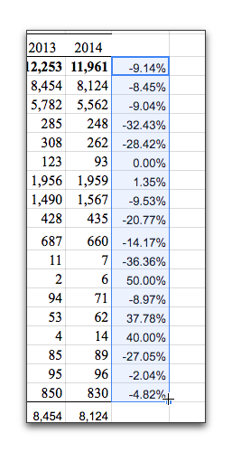
Apply to the rest of the cells

Now let’s apply this percent change formula to the rest of the murder-by-weapon numbers. Click on cell:

G5

Pass your mouse over the bottom right corner of the cell until the cursor changes to thin crosshairs.

Click and drag the mouse cursor down over the rest of the cells in the H column. Release your mouse button when you get to cell:

G22

The percent changes for all the different types of weapons used in homicides will appear on your screen.

Parentheses in a Formula

In the formula for percent change we used in the previous section, parentheses ( ) were included in the formula:

=(F5-B5)/B5

The parentheses in this formula are very important. These tell the spreadsheet to subtract the number of homicides in 2010 (B5) from the number of homicides in 2014 (F5) first, and then divide that amount by the number of homicides in 2010 (B5).

If you didn’t include the parentheses and had just typed in =F5-B5/B5, the spreadsheet first would divide B5 by B5 (yielding 1). Finally it would subtract the result from F5, resulting in an incorrect number.

So if you are doing a calculation involving several steps, it is important to include parentheses so you can group the numbers properly and the spreadsheet thus knows the order in which to do the calculations.

Using Formulas with a Fixed Cell

Another feature you can do with a spreadsheet is building a formula with a fixed cell, so that when you drag your formula to apply them to other cells, it doesn’t automatically switch its reference to a new cell.

In our spreadsheet, for example, we might want to know what percentage of homicides involved each different type of weapon compared to a specific year. We would compare each cell to the total number of homicides for only that year, so we don’t want the reference to that year’s total to change.

Let’s start with 2014. To create our percent formula click on cell:

H6

And type in this formula:

=F6/F5

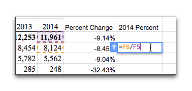
This formula tells the spreadsheet to divide the number of homicides involving firearms in 2010 (F6) by the total number of homicides that year (F5).

Press the enter/return key and swith the cell format to percentage. You’ll see the total is:

67.92%

So firearm related homicides were about two thirds of the total number of homicides in 2014. Good… so far.

But, you might then try to apply this same formula to the cells for the other types of weapons by dragging the crosshairs, as we did in the previous example. But if you tried this, it would produce bizarre numbers in the G column, including that some weapons-related homicides are more than 100% of the total.

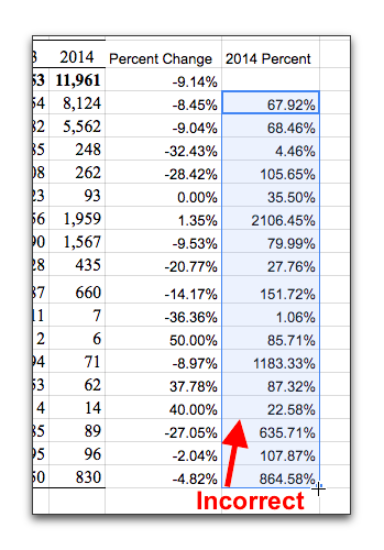
What went wrong?

The problem is that when the spreadsheet copies a formula using this method, it shifts the letters for both cells in the original formula (F6 and F5) as it applies that formula to other cells (resulting in F7 divided by F6 in the next cell down).

To fix this, we need to force the spreadsheet to always divide the numbers for each type of weapon used by a constant number – the total number of homicides in cell F5. This is called anchoring the cell in our formula, and force the spreadsheet always to use one cell each time.

You accomplish this by adding some $ signs to the formula that instruct the spreadsheet not to change cell F5 when applying the formula to other cells.

So go back and click on cell:

F6

Delete that formula (press delete key), and instead type in this:

=F6/$F$5

The dollar signs tell Excel to always keep anchored on cell F5 and the data in it when applying this formula to other cells.

Now we can drag the formula down through the column of cells and get the correct results.

So hover your mouse over cell:

F6

Then click on the crosshairs in the bottom right corner of the cell and drag down to cell:

F22

And release your mouse.

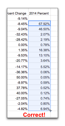
The correct percentage figure for each weapon type will now appear in the spreadsheet.

Adding Numbers Using the SUM Formula

If you want to add a large group of numbers in a row or column, there’s another way to do that quickly in a spreadsheet by using the SUM formula.

For example, in our example spreadsheet on weapons used in homicides, what if you wanted to know the total number of homicides in which did not include a firearm?

To calculate that, you could add up the numbers in rows 12 to 21 for each year using the SUM formula

(Note: row 22 – “Other weapons or weapons not stated” – may or may not involve a non-firearm-related homicide, so we’re leaving that out of this calculation)

To use the SUM formula to calculate the number of non-firearm-related homicides in rows 12 to 21, first click on cell:

B23

In that cell type this formula

=SUM(B12:B21)

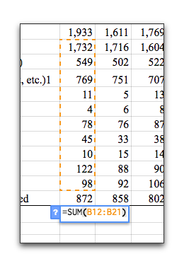
You’ll see there were 3,418 non-firearm-related homicides in 2014. In our formula, =SUM() is shorthand for telling a spreadsheet to add up a series of numbers.

After typing =SUM, you type a set of parentheses, and inside the parenthesis you will include something called a range.

A range has two cell references separated by a colon. B12:B21. Ranges can even span multiple row or multiple columns, and can be used in numerous formulas.

Adding selected cells with the SUM formula instead of a range

You also can add up select numbers in a column, rather than a span of them, using the SUM formula.

To do that, in the SUM formula you replace the colon with commas to separate the specific cells you want to total up.

Thus if you wanted to total up only the number of homicides in 2014 in which either poison (cell B15) or narcotics (cell B18) was involved, you would type this formula.

=SUM(B15,B18)

Shortcuts to Writing Formulas

There are a number of shortcuts for writing formulas in a spreadsheet.

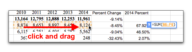
To illustrate these, in our spreadsheet on types of weapons used in homicides, let’s add up the total number of firearm-related homicides from 2010 to 2014. This would mean adding cells B6 through F6. We could manually type in the =SUM(B6:F6) formula, but there is a more user-friendly tool for doing this without having to remember formulas.

To do this, first click on cell:

I6

Then use the spreadsheet’s Formulas tool that will shorten what you have to type.

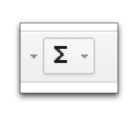
Click on it and you’ll see a series of formulas you can select to insert into your spreadsheet.

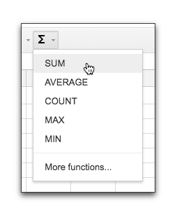
In this case pick SUM and the formula =SUM() will be inserted into cell G6.

Now you can click the cells you want to be referenced, and they will be auto-populated into the formula. You can click-and-drag to specify a range, or click and hold down the shift key and click another cell. To specify specific cells to add without making it a range, you should hold down the command key (Mac) or Control key (PC) and click all the cells you want.

Averaging Numbers

Another common calculation is averaging a series of numbers.

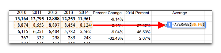
In our spreadsheet on the types of weapons used in homicides, for example, what if we wanted to know the average number of firearm-related homicides each year between 2010 and 2014 (cells B6 to F6).

To do this, click on cell:

J6

And in that cell type:

=AVERAGE(B6:F6)

This same process can be used to also calculate the MEDIAN(), MODE(), STDEV() (standard deviation) and other statistical functions for a series of data points.

Using Functions to Import Website Data

One advantage to Google spreadsheets is that it is designed to work with the Web. Specific functions allow you to load data dynamically directly from a website.

Import a data file published on the Web into your spreadsheet

CSV files (comma separated values) can be imported directly into a spreadsheet from anywhere on the Web. CSV is one of the most common data formats and can be found with a simple Google search.

For sample data, we will use a piece of crime data from UC Berkeley in 2015 hosted on Github. The url is https://raw.githubusercontent.com/jrue/ucpd-crime/master/data/ucpd/ucpd_data_6.csv.

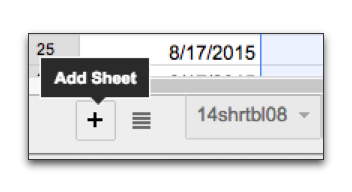
Let’s import this data into a new sheet. Click the small plus button at the bottom of our workbook document:

Click in cell A1 and type (or copy-and-paste) the following:

=ImportData("https://raw.githubusercontent.com/jrue/ucpd-crime/master/data/ucpd/ucpd_data_6.csv")

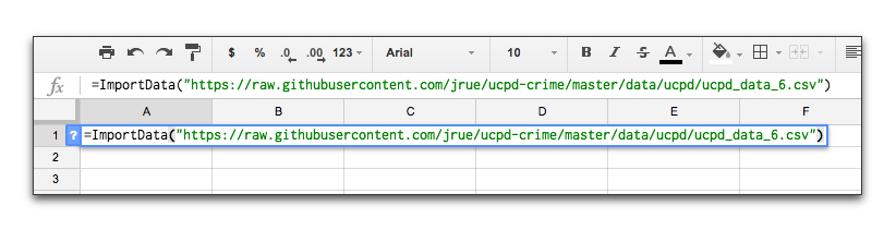
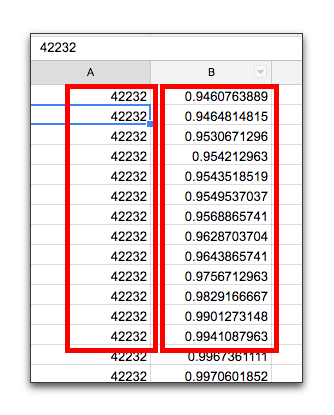
After a moment the data will load and should look like this:

Many files will not be this clean and may require cleanup. But if you can use the file as is, it’s especially useful. Governments regularly update CSV files on their servers. This may happen frequently with certain files such as election results.

Adjusting Data Display by Changing Cell Formats

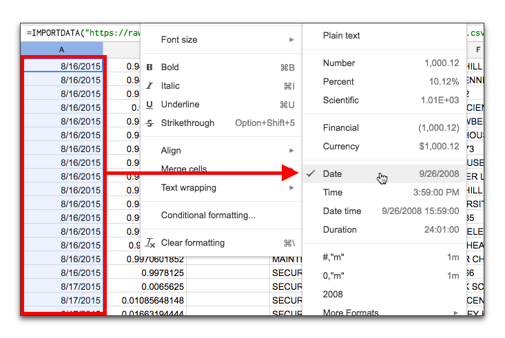
In the previous example, you might have noticed the date and time columns display these strange numbers which should be dates and times of each crime. Raw cell data for a time value is the number of days since Jan 1, 1900 (and may even be different when using Microsoft Excel).

We can easily adjust this by changing the cell format. Click on the column’s heading, then under the Format menu, select Date for the first column, and a Time for the second column.

Import a table or list directly from a Web page

Tables can frequently be imported directly from a Web page into a spreadsheet. Let’s import the same data from the Wikipedia’s page on Gun Violence by State.

Note: This example will tie into the next section on charts, so we use it for convenience. However, we do not advocate using data from Wikipedia in any production sense. Always vet and corroborate data directly from the source when used in journalism.

Open a new sheet and click in cell A1. Type:

=IMPORTHTML("https://en.wikipedia.org/wiki/Gun_violence_in_the_United_States_by_state", "table", 1)

The first parameter is the webpage Google will scan (make sure it’s in quotes). The second parameter is the HTML element it’s looking for. In our case, we want it to find a <table> element. The third parameter is which table element we should find, in case there are multiple. You may need to change the third parameter through trial-and-error, or look at the source code of the webpage you’re scrapping.

Hit enter and the spreadsheet should look like this:

The “table” parameter can be replaced with “list” so that it will look for the contents of <ul> <ol> and <dl> tags.

Load Dynamic Financial Data

Live data from Google finance can be imported into your spreadsheet. The data updates automatically every time the spreadsheet is loaded. Quotes can have up to a 20 minute delay, which is common for financial data.

Create a new spreadsheet that looks like this:

Type =GoogleFinance(".DJI", "price") in cell B2

Type =GoogleFinance(".INX", "price") in cell B3

Type =GoogleFinance(".IXIC", "price") in cell B4

The initials at the beginning of the parentheses are stock ticker symbols. You can find the symbol for any stock at Google Finance.

The cells should update in a few moments and your spreadsheet should look like this:

Load historic financial data

The same function can be used to load historic data. Let’s pull in the daily closing price of Google stock for 2009.

Create a new spreadsheet.

In cell A1, type:

=GoogleFinance("GOOG", "close", "01/01/2009" , "12/31/2009", "DAILY")

Hit enter and the daily closes for 2009 should load into your spreadsheet.

The full documentation on all of the different parameters for the GoogleFinance function are listed on Google’s help pages.

Sorting Results

After you’ve entered numbers or done calculations in a spreadsheet, you may want to sort the results from highest to lowest or lowest to highest.

With the spreadsheet on types of weapons used in homicides, for example, you could more easily see which weapons are most frequently used by ranking them from the highest number to the lowest number for any given year.

To do this, you first need to highlight the area of the spreadsheet that you want to sort.

Don’t just highlight a whole column of numbers to sort because the spreadsheet then will sort only the cells in that column and not change the order of the corresponding cells in other columns (such as the headings that tell you which type of weapon corresponds with the numbers of homicides).

The highlighted area now includes the headings for the types of weapons used and then the numbers for each type of weapon for each year.

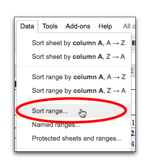
To sort the data, in the menu at the top, click on Data … Sort Range

In the box that appears, you’ll see the range of selected cells displayed at the top (in this case, cells A5 to F22).

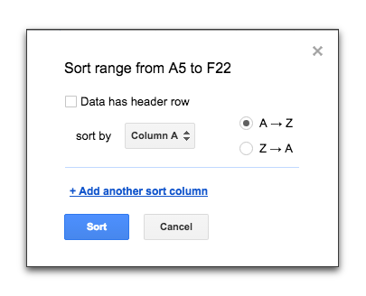
You now can select the column by which you want to sort the data.

You also can select whether to sort that data in ascending order (A – Z) so the smallest number appears at the top of the sorted data, or descending order (Z – A) so the largest number appears at the top.

Formatting Cells

A spreadsheet provides a lot of options for re-formatting the information being displayed. These are similar to the options in a word processing program like Microsoft Word or many other applications. They include:

• Changing the font size or style
• Defining the format for the kind of data in a cell, such as dates, times, currency or percents
• Changing the number of decimal places displayed in a number
• Changing the text color or the background color
• Adding borders around the cells

Some of these options are available by selecting Format in the menu at the top and then picking one of the choices in the drop-down menu.

Or you can click on the icons in the middle of the toolbar for other options.