How to make a Bar Chart in D3
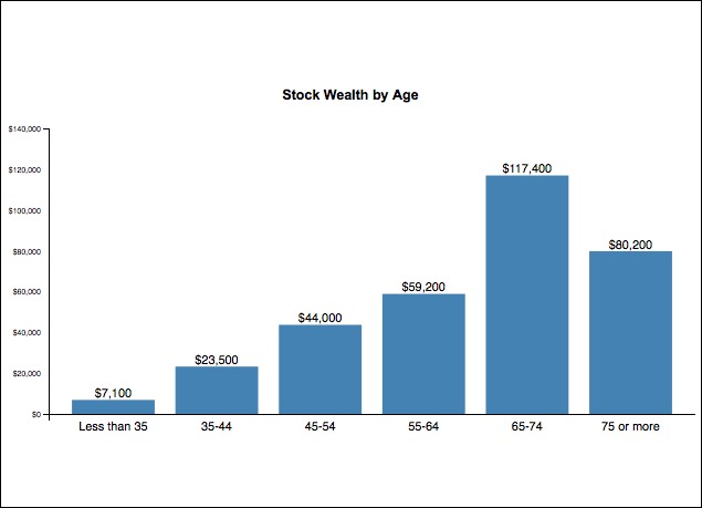
Basic Bar Chart
Step 1: Prepare your data as a CSV file
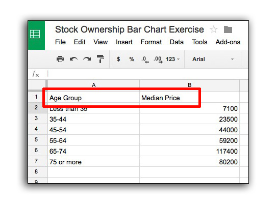
Make sure your data are real numbers, and have no commas or symbols in them (decimals are OK).
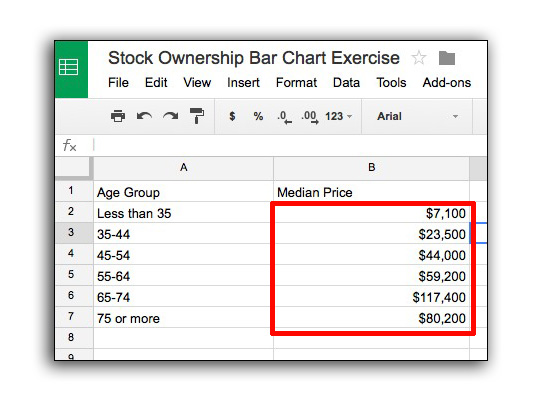
Note, that the headers of your spreadsheet will become properties of your data when you bring it in.
To access each piece of data, the following notation would be used:
data[0]["Age Group"] //will return "Less than 35"
data[1]["Age Group"] //will return "35-44"
data[2]["Age Group"] //will return "45-54"
data[3]["Age Group"] //will return "55-64"
//...and so on

data[0]["Median Price"] //will return "7100"
data[1]["Median Price"] //will return "23000"
data[2]["Median Price"] //will return "44000"
data[3]["Median Price"] //will return "59200"
//...and so on
Save your spreadsheet as a .csv file in a folder where you will put the html for your bar chart.
Step 2: Create your HTML file
Here is a basic boilerplate template with the D3 library included to start you off. Save this with the .html file extension in the same folder as your .csv file.
<!DOCTYPE html>
<html>
<head>
    <meta charset="utf-8">
    <title>Basic Bar Chart</title>
    <meta http-equiv="X-UA-Compatible" content="IE=edge,chrome=1">
    <meta name="viewport" content="width=device-width, initial-scale=1">
    <style>
    /* custom css styles will go here */

    </style>
</head>
<body>

    <script src="https://d3js.org/d3.v5.min.js"></script>
    <script>
        //your d3 code will go here


    </script>
</body>
</html>
Step 3: Setup your size variables and your SVG
Next, setup some basic size variables for our SVG container.
var margin = {top:0, right:0, bottom:20, left:50},
    width  = 800 - margin.left - margin.right,
    height = 500 - margin.top - margin.bottom;

var svg = d3.select("body")
    .append("svg")
    .attr("width", "100%")
    .attr("height", "100%")
    .attr("viewBox", "0 0 " + (width + margin.left + margin.right) + " " + (height + margin.top + margin.bottom));

var chart = svg.append("g")
    .attr("transform", "translate(" + margin.left + "," + margin.top + ")");
The viewBox attribute specifies the internal coordinate system for your chart using an x y width height format. This way you can set the width and height to 100%, and your chart will become responsive.
Step 4: Set your scales
Next, set the scales for the X and Y axis. For a column bar chart chart, your X scale will be determined the number of elements you have, and your Y scale will be determined the maximum value of your data.
We also subtract the margins, since these will add space for our axes and any labels we decide to add.
var yScale = d3.scaleLinear()
    .range([height, 0]);

var xScale = d3.scaleBand()
    .range([0, width])
    .padding(0.1);
As a reminder, .scaleBand() is a special bar-chart function to make the bars clean and spaced properly.
Step 5: Running a Python SimpleHTTPServer
NOTE: This step is not required if using a code editor like Brackets.io, which comes with a built-in web server.
For Macs, you can launch the Terminal program, navigate to the folder where your project is using terminal commands cd (tutorial here), then run the following command:
python -m SimpleHTTPServer 8000
Step 6: Loading in the CSV file using D3
Next, we load in the CSV file.
d3.csv("stockowners.csv").then(function(data){
    //code in next sections will go here.


});
Step 7: Coercing the strings as numbers
D3 pulls in data as strings, even when they’re numbers. You can convert your data so that the strings will be recast as numbers.
//map function goes through every element, then returns a number for median price
data = data.map(function(d){
    d["Median Price"] = +d["Median Price"];
    return d;
});
Step 8: Setting the domains for the X and Y scales
Since we are loading in our data via CSV, we can’t set the domains until the data is loaded in. After we load in the data and coerce as numbers, we can set our domains. Our X scale simply needs unique strings for each element in the data (in our case, Age Group), and our Y scale need a domain from zero to the maximum value.
In each situation, we map the data from the array of objects. The d3.max() function will allow us to find the maximum piece of data in the array. Inside the return function, we have to specify which property (“Median Price”, or “Age Group”) we want to extract the max or minimum values.
//yscale's domain is from zero to the maximum "Median Price" in your data
yScale.domain([0, d3.max(data, function(d){ return d["Median Price"]; })]);

//xscale is unique values in your data (Age Group, since they are all different)
xScale.domain(data.map(function(d){ return d["Age Group"]; }));
Step 9: Creating the Bar Chart
Next, we run through our data and build the bar chart. We will add the bar chart to a grouping “g” element so that we can account for margins. It’s important to add a class name to each bar so that we can style it with CSS.
chart.selectAll(".bar")
    .data(data)
    .enter()
    .append("rect")
    .attr("class", "bar")
    .attr("x", function(d){ return xScale(d["Age Group"]); })
    .attr("y", function(d){ return yScale(d["Median Price"]); })
    .attr("height", function(d){ return height - yScale(d["Median Price"]); })
    .attr("width", function(d){ return xScale.bandwidth(); })
    .attr("fill", "steelblue");
Step 10: Adding the axes
To add the axes, append a “g” group element, and use the transform attribute to position it in the correct location accounting for the margins. Then call either the xAxis or yAxis functions you created earlier.
We also add two class names so we can style each axis individually.
Note that we added .tickFormat(d3.format("$,")) line after the scale to include a dollar symbol before the number, and comma-separate the number by thousands. This is part of what’s called SI Prefix code. More documentation on what’s possible can be found on the d3 site.
//adding y axis to the left of the chart
svg.append("g")
    .attr("transform", "translate(" + margin.left + "," + margin.top + ")")
    .call(d3.axisLeft(yScale).tickFormat(d3.format("$,")));

//adding x axis to the bottom of chart
svg.append("g")
    .attr("transform", "translate(" + margin.left + "," + (height + margin.top) + ")")
    .call(d3.axisBottom(xScale));
Step 11 (Optional): Make adjustments
Once your data is in and you see your chart, you may wish to make some adjustments so that the graph can communicate effectively. You can make adjustments to your domain on your yScale, for example, so that the maximum value isn’t all the way at the top.
//increasing domain to static 140000, so it's more than maximum value in your data
yScale.domain([0, 140000]);
It’s also possible to add labels at the top of each bar by running through the data again. (Another more efficient way would have been to create a grouping for each bar then append text to that).
Here we use the same X and Y scales to place each text label above the bars.
//add text labels to the top of each bar
svg.append("g")
    .attr("transform", "translate(" + margin.left + "," + margin.top + ")")
    .selectAll(".textlabel")
    .data(data)
    .enter()
    .append("text")
    .attr("class", "textlabel")
    .attr("x", function(d){ return xScale(d["Age Group"]) + (xScale.bandwidth()/2); })
    .attr("y", function(d){ return yScale(d["Median Price"]) - 3; })
    .attr("text-anchor", "middle")
    .attr("font-family", "sans-serif")
    .attr("font-size", "10px")
    .text(function(d){ return d3.format("$,")(d["Median Price"]); });
    //more info about d3 format method:
    // http://koaning.s3-website-us-west-2.amazonaws.com/html/d3format.html
You can also adjust the padding to account for a label at the top.
//add additional top margin to make room for label
var margin = {top:50, right:0, bottom:20, left:50};
Then add the title at the top. We use width divided by 2, to center (make sure the text-anchor is set to middle for the CSS styling to properly center the text).
//adding a label at the top of the chart
svg.append("g")
    .attr("transform", "translate(" + (width/2) + ", 15)")
    .append("text")
    .text("Stock Wealth by Age")
    .style("text-anchor", "middle")
    .style("font-family", "Arial")
    .style("font-weight", "800");
FINAL CODE
Here is the entire code in one block. NOTE: This requires the stockowners.csv file in the same folder. This project will only work if you run it from a webserver.
<!DOCTYPE html>
<html>
<head>
    <meta charset="utf-8">
    <title>Basic Bar Chart</title>
    <meta http-equiv="X-UA-Compatible" content="IE=edge,chrome=1">
    <meta name="viewport" content="width=device-width, initial-scale=1">
    <style type="text/css">
    /* custom css styles will go here */

    </style>
</head>
<body>

    <script src="https://d3js.org/d3.v5.min.js"></script>
    <script>
      var margin = {top:0, right:0, bottom:20, left:50},
          width  = 800 - margin.left - margin.right,
          height = 500 - margin.top - margin.bottom;

      var svg = d3.select("body")
          .append("svg")
          .attr("width", "100%")
          .attr("height", "100%")
          .attr("viewBox", "0 0 " + (width + margin.left + margin.right) + " " + (height + margin.top + margin.bottom));

      var chart = svg.append("g")
          .attr("transform", "translate(" + margin.left + "," + margin.top + ")");

      var yScale = d3.scaleLinear()
          .range([height, 0]);

      var xScale = d3.scaleBand()
          .range([0, width])
          .padding(0.1);

      d3.csv("stockowners.csv").then(function(data){

        data = data.map(function(d){
            d["Median Price"] = +d["Median Price"];
            return d;
        });

        yScale.domain([0, d3.max(data, function(d){ return d["Median Price"]; }) + 10000]);
        xScale.domain(data.map(function(d){ return d["Age Group"]; }));

        chart.selectAll(".bar")
            .data(data)
            .enter()
            .append("rect")
            .attr("class", "bar")
            .attr("x", function(d){ return xScale(d["Age Group"]); })
            .attr("y", function(d){ return yScale(d["Median Price"]); })
            .attr("height", function(d){ return height - yScale(d["Median Price"]); })
            .attr("width", function(d){ return xScale.bandwidth(); })
            .attr("fill", "steelblue");

        svg.append("g")
            .attr("transform", "translate(" + margin.left + "," + margin.top + ")")
            .selectAll(".textlabel")
            .data(data)
            .enter()
            .append("text")
            .attr("class", "textlabel")
            .attr("x", function(d){ return xScale(d["Age Group"]) + (xScale.bandwidth()/2); })
            .attr("y", function(d){ return yScale(d["Median Price"]) - 3; })
            .attr("text-anchor", "middle")
            .attr("font-family", "sans-serif")
            .attr("font-size", "10px")
            .text(function(d){ return d3.format("$,")(d["Median Price"]); });

        //adding y axis to the left of the chart
        svg.append("g")
            .attr("transform", "translate(" + margin.left + "," + margin.top + ")")
            .call(d3.axisLeft(yScale).tickFormat(d3.format("$,")));

        //adding x axis to the bottom of chart
        svg.append("g")
            .attr("transform", "translate(" + margin.left + "," + (height + margin.top) + ")")
            .call(d3.axisBottom(xScale));

        svg.append("g")
            .attr("transform", "translate(" + (width/2) + ", 15)")
            .append("text")
            .text("Stock Wealth by Age")
            .style("text-anchor", "middle")
            .style("font-family", "Arial")
            .style("font-weight", "800");
      });
    </script>
</body>
</html>